Approach of the Method in A Small Sample
Selcen Ari
2019-10-17
Source:vignettes/small_sample.Rmd
small_sample.RmdInstallation of ceRNAnetsim
#install.packages("devtools")
#devtools::install_github("selcenari/ceRNAnetsim")

library(ceRNAnetsim)
Load the minimal sample
In this vignette, the model functions are demonstrated with minimal sample dataset. Dataset minsamp includes miRNA:target interaction factors in addition to basic_data in basic usage of package. minsamp is a sample dataset that includes 6 genes, 2 miRNAs and interaction factors of miRNA:gene pairs.
data("minsamp")

minsamp
#>   competing miRNA Competing_expression miRNA_expression seed_type region
#> 1     Gene1  Mir1                10000             1000      0.43   0.30
#> 2     Gene2  Mir1                10000             1000      0.43   0.01
#> 3     Gene3  Mir1                 5000             1000      0.32   0.40
#> 4     Gene4  Mir1                10000             1000      0.23   0.50
#> 5     Gene4  Mir2                10000             2000      0.35   0.90
#> 6     Gene5  Mir2                 5000             2000      0.05   0.40
#> 7     Gene6  Mir2                10000             2000      0.01   0.80
#>   energy
#> 1    -20
#> 2    -15
#> 3    -14
#> 4    -10
#> 5    -12
#> 6    -11
#> 7    -25
Convert the dataset to graph
minimal sample minsamp is processed with priming_graph() function in first step. This provides conversion of dataset from data frame to graph object. This step comprises of:
- The competing elements (Genes in minsamp) are grouped according to the miRNAs they are associated with.
- In graph object, the optional interaction factors are processed and graded within the groups.
- The amounts (expressions) of miRNAs are distributed according to competing:total competing ratio.
- miRNA efficiency in steady-state is calculated by taking into account of expression distribution and effecting factors. The optional factors might have two types of effect; 1) affinity, 2) degradation effect. Any column which has effect on affinity should be provided as a vector to
aff_factorargument and any column that effects degradation of target RNA should be as a vector todeg_factorargument.
priming_graph(minsamp,
              competing_count = Competing_expression,
              miRNA_count = miRNA_expression,
              aff_factor = c(energy, seed_type),
              deg_factor = region)
#> Warning in priming_graph(minsamp, competing_count = Competing_expression, : First column is processed as competing and the second as miRNA.
#> # A tbl_graph: 8 nodes and 7 edges
#> #
#> # A rooted tree
#> #
#> # Node Data: 8 x 7 (active)
#>   name  type  node_id initial_count count_pre count_current
#>   <chr> <chr>   <int>         <dbl>     <dbl>         <dbl>
#> 1 Gene1 Comp~       1         10000     10000         10000
#> 2 Gene2 Comp~       2         10000     10000         10000
#> 3 Gene3 Comp~       3          5000      5000          5000
#> 4 Gene4 Comp~       4         10000     10000         10000
#> 5 Gene5 Comp~       5          5000      5000          5000
#> 6 Gene6 Comp~       6         10000     10000         10000
#> # ... with 2 more rows, and 1 more variable: changes_variable <chr>
#> #
#> # Edge Data: 7 x 22
#>    from    to Competing_name miRNA_name Competing_expre~ miRNA_expression
#>   <int> <int> <chr>          <chr>                 <dbl>            <dbl>
#> 1     1     7 Gene1          Mir1                  10000             1000
#> 2     2     7 Gene2          Mir1                  10000             1000
#> 3     3     7 Gene3          Mir1                   5000             1000
#> # ... with 4 more rows, and 16 more variables: energy <dbl>,
#> #   seed_type <dbl>, region <dbl>, dummy <dbl>, afff_factor <dbl>,
#> #   degg_factor <dbl>, comp_count_list <list>, comp_count_pre <dbl>,
#> #   comp_count_current <dbl>, mirna_count_list <list>,
#> #   mirna_count_pre <dbl>, mirna_count_current <dbl>,
#> #   mirna_count_per_dep <dbl>, effect_current <dbl>, effect_pre <dbl>,
#> #   effect_list <list>
In the processed data, the values are carried as node variables and many more columns are initialized which are to be used in subsequent steps.
Change expression level of one or more nodes in the graph
In the steady-state, the miRNA degradation effect on gene expression is assumed to be stable (i.e. in equilibrium). But, if one or more nodes have altered expression level, the system tends to reach steady-state again.
The ceRNAnetsim package utilizes two methods to simulate change in expression level, update_how() and update_variables() functions provide unstable state from which calculations are triggered to reach steady-state.
Method 1: change expression level of single node
If updating expression level of single node is desired then update_how() function should be used. In the example below, expression level of Gene4 is increased 2-fold.
minsamp %>%
   priming_graph(competing_count = Competing_expression,
                 miRNA_count = miRNA_expression,
                 aff_factor = c(energy, seed_type),
                 deg_factor = region) %>%
   update_how(node_name = "Gene4", how = 2) %>%
   activate(edges)%>%
   # following line is just for focusing on necessary
   # columns to see the change in edge data
   select(3:4,comp_count_pre,comp_count_current)
#> Warning in priming_graph(., competing_count = Competing_expression, miRNA_count = miRNA_expression, : First column is processed as competing and the second as miRNA.
#> # A tbl_graph: 8 nodes and 7 edges
#> #
#> # A rooted tree
#> #
#> # Edge Data: 7 x 6 (active)
#>    from    to Competing_name miRNA_name comp_count_pre comp_count_current
#>   <int> <int> <chr>          <chr>               <dbl>              <dbl>
#> 1     1     7 Gene1          Mir1                10000              10000
#> 2     2     7 Gene2          Mir1                10000              10000
#> 3     3     7 Gene3          Mir1                 5000               5000
#> 4     4     7 Gene4          Mir1                10000              20000
#> 5     4     8 Gene4          Mir2                10000              20000
#> 6     5     8 Gene5          Mir2                 5000               5000
#> # ... with 1 more row
#> #
#> # Node Data: 8 x 7
#>   name  type  node_id initial_count count_pre count_current
#>   <chr> <chr>   <int>         <dbl>     <dbl>         <dbl>
#> 1 Gene1 Comp~       1         10000     10000         10000
#> 2 Gene2 Comp~       2         10000     10000         10000
#> 3 Gene3 Comp~       3          5000      5000          5000
#> # ... with 5 more rows, and 1 more variable: changes_variable <chr>
Method 2: update expression level of all nodes
The update_variables() function uses an external dataset which has number of rows equal to number of nodes in graph. The external dataset might include changed and unchanged expression values for each node.
Load the new_count dataset (provided with package sample data) in which expression level of Gene2 is increased 2 fold (from 10,000 to 20,000). Note that variables of the dataset included updated variables must be named as “Competing”, “miRNA”, “miRNA_count” and “Competing_count”.
data(new_counts)
new_counts
#>   Competing miRNA Competing_count miRNA_count
#> 1     Gene1  Mir1           10000        1000
#> 2     Gene2  Mir1           20000        1000
#> 3     Gene3  Mir1            5000        1000
#> 4     Gene4  Mir1           10000        1000
#> 5     Gene4  Mir2           10000        2000
#> 6     Gene5  Mir2            5000        2000
#> 7     Gene6  Mir2           10000        2000
update_variables() function replaces the existing expression values with new values. The function checks for updates in all rows after importing expression values, thus it’s possible to introduce multiple changes at once.
minsamp %>%
   priming_graph(competing_count = Competing_expression,
                 miRNA_count = miRNA_expression,
                 aff_factor = c(energy, seed_type),
                 deg_factor = region) %>%
   update_variables(current_counts = new_counts)
#> Warning in priming_graph(., competing_count = Competing_expression, miRNA_count = miRNA_expression, : First column is processed as competing and the second as miRNA.
#> # A tbl_graph: 8 nodes and 7 edges
#> #
#> # A rooted tree
#> #
#> # Node Data: 8 x 7 (active)
#>   name  type  node_id initial_count count_pre count_current
#>   <chr> <chr>   <int>         <dbl>     <dbl>         <dbl>
#> 1 Gene1 Comp~       1         10000     10000         10000
#> 2 Gene2 Comp~       2         10000     10000         20000
#> 3 Gene3 Comp~       3          5000      5000          5000
#> 4 Gene4 Comp~       4         10000     10000         10000
#> 5 Gene5 Comp~       5          5000      5000          5000
#> 6 Gene6 Comp~       6         10000     10000         10000
#> # ... with 2 more rows, and 1 more variable: changes_variable <chr>
#> #
#> # Edge Data: 7 x 22
#>    from    to Competing_name miRNA_name Competing_expre~ miRNA_expression
#>   <int> <int> <chr>          <chr>                 <dbl>            <dbl>
#> 1     1     7 Gene1          Mir1                  10000             1000
#> 2     2     7 Gene2          Mir1                  10000             1000
#> 3     3     7 Gene3          Mir1                   5000             1000
#> # ... with 4 more rows, and 16 more variables: energy <dbl>,
#> #   seed_type <dbl>, region <dbl>, dummy <dbl>, afff_factor <dbl>,
#> #   degg_factor <dbl>, comp_count_list <list>, comp_count_pre <dbl>,
#> #   comp_count_current <dbl>, mirna_count_list <list>,
#> #   mirna_count_pre <dbl>, mirna_count_current <dbl>,
#> #   mirna_count_per_dep <dbl>, effect_current <dbl>, effect_pre <dbl>,
#> #   effect_list <list>
Update the node variables with edge variables.
The functions update_variables() and update_how() updates edge data. In these functions, update_nodes() function is applied in order to reflect changes in edge data over to node data. In other words, if there’s a change in edge data, nodes can be updated accordingly with update_nodes() function.
minsamp %>%
  priming_graph(competing_count = Competing_expression,
                miRNA_count = miRNA_expression,
                aff_factor = c(energy, seed_type),
                deg_factor = region) %>%
  update_how("Gene4", how = 2)
#> Warning in priming_graph(., competing_count = Competing_expression, miRNA_count = miRNA_expression, : First column is processed as competing and the second as miRNA.
#> # A tbl_graph: 8 nodes and 7 edges
#> #
#> # A rooted tree
#> #
#> # Node Data: 8 x 7 (active)
#>   name  type  node_id initial_count count_pre count_current
#>   <chr> <chr>   <int>         <dbl>     <dbl>         <dbl>
#> 1 Gene1 Comp~       1         10000     10000         10000
#> 2 Gene2 Comp~       2         10000     10000         10000
#> 3 Gene3 Comp~       3          5000      5000          5000
#> 4 Gene4 Comp~       4         10000     10000         20000
#> 5 Gene5 Comp~       5          5000      5000          5000
#> 6 Gene6 Comp~       6         10000     10000         10000
#> # ... with 2 more rows, and 1 more variable: changes_variable <chr>
#> #
#> # Edge Data: 7 x 22
#>    from    to Competing_name miRNA_name Competing_expre~ miRNA_expression
#>   <int> <int> <chr>          <chr>                 <dbl>            <dbl>
#> 1     1     7 Gene1          Mir1                  10000             1000
#> 2     2     7 Gene2          Mir1                  10000             1000
#> 3     3     7 Gene3          Mir1                   5000             1000
#> # ... with 4 more rows, and 16 more variables: energy <dbl>,
#> #   seed_type <dbl>, region <dbl>, dummy <dbl>, afff_factor <dbl>,
#> #   degg_factor <dbl>, comp_count_list <list>, comp_count_pre <dbl>,
#> #   comp_count_current <dbl>, mirna_count_list <list>,
#> #   mirna_count_pre <dbl>, mirna_count_current <dbl>,
#> #   mirna_count_per_dep <dbl>, effect_current <dbl>, effect_pre <dbl>,
#> #   effect_list <list>

# OR
# minsamp %>%
#   priming_graph(competing_count = Competing_expression,
#                 miRNA_count = miRNA_expression,
#                 aff_factor = c(energy, seed_type),
#                 deg_factor = region) %>%
# update_variables(current_counts = new_counts) 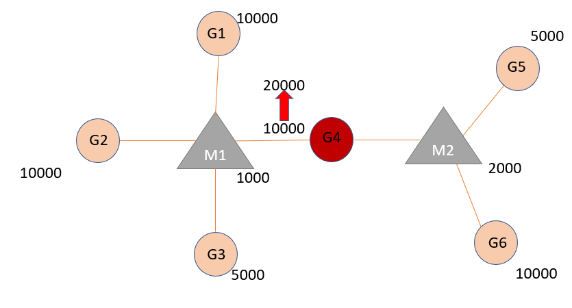
Simulate the model
Change in expression level of one or more nodes will trigger a perturbation in the system which will effect neighboring miRNA:target interactions. The effect will propagate and iterate over until it reaches steady-state.
With simulate() function the changes in the system, are calculated iteratively. For example, in the example below, simulation will proceed ten cycles only. In simulation of the regulation, the important argument is threshold which provides to specify absolute minimum amount of change required to be considered changed element as up or down.
minsamp %>%
  priming_graph(competing_count = Competing_expression,
                miRNA_count = miRNA_expression,
                aff_factor = c(energy, seed_type),
                deg_factor = region) %>%
  update_how("Gene4", how = 2) %>%
  simulate(cycle=10) #threshold with default 0.
#> Warning in priming_graph(., competing_count = Competing_expression, miRNA_count = miRNA_expression, : First column is processed as competing and the second as miRNA.
#> # A tbl_graph: 8 nodes and 7 edges
#> #
#> # A rooted tree
#> #
#> # Node Data: 8 x 7 (active)
#>   name  type  node_id initial_count count_pre count_current
#>   <chr> <chr>   <int>         <dbl>     <dbl>         <dbl>
#> 1 Gene1 Comp~       1         10000    10027.        10027.
#> 2 Gene2 Comp~       2         10000    10001.        10001.
#> 3 Gene3 Comp~       3          5000     5009.         5009.
#> 4 Gene4 Comp~       4         10000    19806.        19806.
#> 5 Gene5 Comp~       5          5000     5024.         5024.
#> 6 Gene6 Comp~       6         10000    10044.        10044.
#> # ... with 2 more rows, and 1 more variable: changes_variable <chr>
#> #
#> # Edge Data: 7 x 23
#>    from    to Competing_name miRNA_name Competing_expre~ miRNA_expression
#>   <int> <int> <chr>          <chr>                 <dbl>            <dbl>
#> 1     1     7 Gene1          Mir1                  10000             1000
#> 2     2     7 Gene2          Mir1                  10000             1000
#> 3     3     7 Gene3          Mir1                   5000             1000
#> # ... with 4 more rows, and 17 more variables: energy <dbl>,
#> #   seed_type <dbl>, region <dbl>, dummy <dbl>, afff_factor <dbl>,
#> #   degg_factor <dbl>, comp_count_list <list>, comp_count_pre <dbl>,
#> #   comp_count_current <dbl>, mirna_count_list <list>,
#> #   mirna_count_pre <dbl>, mirna_count_current <dbl>,
#> #   mirna_count_per_dep <dbl>, effect_current <dbl>, effect_pre <dbl>,
#> #   effect_list <list>, mirna_count_per_comp <dbl>
simulate() saves the expression level of previous iterations in list columns in edge data. The changes in expression level throughout the simulate cycles are accessible with standard dplyr functions. For example:
minsamp %>%
   priming_graph(competing_count = Competing_expression,
                 miRNA_count = miRNA_expression,
                 aff_factor = c(energy, seed_type),
                 deg_factor = region) %>%
   update_how("Gene4", how = 2) %>%
   simulate(cycle=10) %>%
   activate(edges) %>%       #from tidygraph package
   select(comp_count_list, mirna_count_list) %>%
   as_tibble()
#> Warning in priming_graph(., competing_count = Competing_expression, miRNA_count = miRNA_expression, : First column is processed as competing and the second as miRNA.
#> # A tibble: 7 x 4
#>    from    to comp_count_list mirna_count_list
#>   <int> <int> <list>          <list>
#> 1     1     7 <dbl [11]>      <dbl [11]>
#> 2     2     7 <dbl [11]>      <dbl [11]>
#> 3     3     7 <dbl [11]>      <dbl [11]>
#> 4     4     7 <dbl [11]>      <dbl [11]>
#> 5     4     8 <dbl [11]>      <dbl [11]>
#> 6     5     8 <dbl [11]>      <dbl [11]>
#> 7     6     8 <dbl [11]>      <dbl [11]>
Here, comp_count_list and mirna_count_list are list-columns which track changes in both competing RNA and miRNA levels. In the sample above, “Gene4” has initial expression level of 10000 (after trigger, it’s initial expression is 20000) and reached level of 19806 at 9th cycle (count_pre) and also stayed at 19806 in last cycle (count_current). The full history of expression level for Gene4 is as follows:
#> [1] 10000 19803 19806 19806 19806 19806 19806 19806 19806 19806 19806Actually, Gene4 seems like reached steady-state in iteration 4. But, this approach is sensitive to even small decimal numbers. So, threshold argument could be used to ignore very small decimal numbers. With a threshold value the system can reach steady-state early, like following.
minsamp %>%
  priming_graph(competing_count = Competing_expression,
                miRNA_count = miRNA_expression,
                aff_factor = c(energy, seed_type),
                deg_factor = region) %>%
  update_how("Gene4", how = 2) %>%
  simulate(cycle=3, threshold = 1)
#> Warning in priming_graph(., competing_count = Competing_expression, miRNA_count = miRNA_expression, : First column is processed as competing and the second as miRNA.
#> # A tbl_graph: 8 nodes and 7 edges
#> #
#> # A rooted tree
#> #
#> # Node Data: 8 x 7 (active)
#>   name  type  node_id initial_count count_pre count_current
#>   <chr> <chr>   <int>         <dbl>     <dbl>         <dbl>
#> 1 Gene1 Comp~       1         10000    10027.        10027.
#> 2 Gene2 Comp~       2         10000    10001.        10001.
#> 3 Gene3 Comp~       3          5000     5009.         5009.
#> 4 Gene4 Comp~       4         10000    19806.        19806.
#> 5 Gene5 Comp~       5          5000     5024.         5024.
#> 6 Gene6 Comp~       6         10000    10044.        10044.
#> # ... with 2 more rows, and 1 more variable: changes_variable <chr>
#> #
#> # Edge Data: 7 x 23
#>    from    to Competing_name miRNA_name Competing_expre~ miRNA_expression
#>   <int> <int> <chr>          <chr>                 <dbl>            <dbl>
#> 1     1     7 Gene1          Mir1                  10000             1000
#> 2     2     7 Gene2          Mir1                  10000             1000
#> 3     3     7 Gene3          Mir1                   5000             1000
#> # ... with 4 more rows, and 17 more variables: energy <dbl>,
#> #   seed_type <dbl>, region <dbl>, dummy <dbl>, afff_factor <dbl>,
#> #   degg_factor <dbl>, comp_count_list <list>, comp_count_pre <dbl>,
#> #   comp_count_current <dbl>, mirna_count_list <list>,
#> #   mirna_count_pre <dbl>, mirna_count_current <dbl>,
#> #   mirna_count_per_dep <dbl>, effect_current <dbl>, effect_pre <dbl>,
#> #   effect_list <list>, mirna_count_per_comp <dbl>
Visualisation of the graph
The vis_graph() function is used for visualization of the graph object. The initial graph object (steady-state) is visualized as following:
minsamp %>%
   priming_graph(competing_count = Competing_expression,
                 miRNA_count = miRNA_expression,
                 aff_factor = c(energy, seed_type),
                 deg_factor = region) %>%
   vis_graph(title = "Minsamp initial Graph")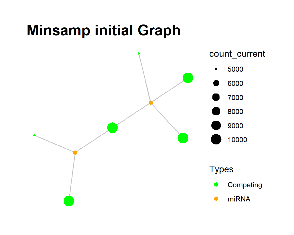
Also, The graph can be visualized at any step of process, for example, after simulation of 3 cycles the graph will look like:
minsamp %>%
   priming_graph(competing_count = Competing_expression,
                 miRNA_count = miRNA_expression,
                 aff_factor = c(energy, seed_type),
                 deg_factor = region) %>%
   update_variables(current_counts = new_counts) %>%
   simulate(3) %>%
   vis_graph(title = "Minsamp Graph After 3 Iteration")
On the other hand, the network of each step can be plotted individually by using simulate_vis() function. simulate_vis() processes the given network just like simulate() function does while saving image of each step.
minsamp %>%
   priming_graph(competing_count = Competing_expression,
                 miRNA_count = miRNA_expression,
                 aff_factor = c(energy, seed_type),
                 deg_factor = region) %>%
   update_variables(current_counts = new_counts) %>%
   simulate_vis(3, title = "Minsamp Graph After Each Iteration")
Minsamp with 3 iteration
Note: Animated gif above was generated by online service. Actually, workflow gives the frames which include condition of each iteration. Note that you must use a terminal or online service, if you want to generate the animated gif.
See the other vignettes for more advanced examples.